User Interface

PyDFT is an educational pure-Python module to perform simple density functional theory (DFT) calculations using a Gaussian basis set. Uniquely, PyDFT exposes many routines that are normally hidden from the user, which are potentially interesting for the user to understand how a DFT calculations is performed. We will provide a demonstration here.

Note

Every code snippet listed below can be run stand-alone. This does imply that every code snippet re-performed the initial self-consistent field calculation. If that is undesirable, the reader is invited to copy the relevant parts of the code (highlighted) and place these in a single file.

Building molecules

Molecules can be built either directly using the Molecule class or via a MoleculeBuilder convenience routine.

Important

The Molecule and MoleculeBuilder classes are not implemented in PyDFT but are obtained from the PyQInt module.

Molecule class

To manually build a molecule, one first need to construct a Molecule object after which one or more atoms can be assigned to the molecule. If no unit is specified, it is assumed that all coordinates are given in atomic units (i.e. Bohr units).

from pyqint import Molecule

mol = Molecule('co')
mol.add_atom('C', 0.0, 0.0, 0.0, unit='angstrom')
mol.add_atom('O', 0.0, 0.0, 1.2, unit='angstrom')

MoleculeBuilder class

Alternatively, a Molecule can be constructed from the MoleculeBuilder class which uses a name. For more information about the MoleculeBuilder class, please consult the PyQInt documentation on the MoleculeBuilder class.

from pyqint import Molecule

co = MoleculeBuilder().from_name("CO")

Calculating electronic energy

To start, we perform a high-level calculation of the electronic structure of the carbon-monoxide molecule using the PBE exchange-correlation functional. To perform this calculation, we first have to construct a pydft.DFT object which requires a molecule as its input. Next, we use the pydft.DFT.scf() routine to start the self-consistent field calculation.

import numpy as np
from pydft import MoleculeBuilder, DFT

# perform DFT calculation on the CO molecule
co = MoleculeBuilder().from_name("CO")
dft = DFT(co, basis='sto3g')
en = dft.scf(1e-6, verbose=False)

# print total energy
print("Total electronic energy:     %12.6f Ht" % en)

Performing this calculation shows that the total electronic energy for this system corresponds to:

Total electronic energy:      -111.147096 Ht

Showing the electronic steps

import numpy as np
from pydft import MoleculeBuilder, DFT

# perform DFT calculation on the CO molecule
co = MoleculeBuilder().from_name("CO")
dft = DFT(co, basis='sto3g')
en = dft.scf(1e-5, verbose=True)

Executing the script above yields the following output:

001 | E =  -179.237380 | dE = 0.0000e+00 | 0.0010 s
002 | E =  -106.678953 | dE = 0.0000e+00 | 0.0810 s
003 | E =  -117.660767 | dE = 7.2558e+01 | 0.0670 s
004 | E =  -107.204261 | dE = 1.0982e+01 | 0.0660 s
005 | E =  -117.396119 | dE = 1.0457e+01 | 0.0610 s
006 | E =  -117.080704 | dE = 1.0192e+01 | 0.0690 s
007 | E =  -108.040074 | dE = 3.1541e-01 | 0.0580 s
008 | E =  -107.453445 | dE = 9.0406e+00 | 0.0620 s
009 | E =  -110.504979 | dE = 5.8663e-01 | 0.0710 s
010 | E =  -110.484364 | dE = 3.0515e+00 | 0.0680 s
011 | E =  -109.605523 | dE = 2.0615e-02 | 0.0680 s
012 | E =  -111.037173 | dE = 8.7884e-01 | 0.0630 s
013 | E =  -111.136251 | dE = 1.4317e+00 | 0.0710 s
014 | E =  -111.147174 | dE = 9.9078e-02 | 0.0730 s
015 | E =  -111.146826 | dE = 1.0923e-02 | 0.0660 s
016 | E =  -111.146838 | dE = 3.4816e-04 | 0.0720 s
017 | E =  -111.146838 | dE = 1.2150e-05 | 0.0660 s
018 | E =  -111.146838 | dE = 8.0277e-08 | 0.0660 s
Stopping SCF cycle, convergence reached.

Different exchange-correlation functionals

To use a different exchange-correlation functional, we can use the

import numpy as np
from pydft import MoleculeBuilder, DFT

# perform DFT calculation on the CO molecule
co = MoleculeBuilder().from_name("CO")

# use SVWM XC functional
dft = DFT(co, basis='sto3g', functional='svwn5')
print('SVWN: ', dft.scf(1e-5), 'Ht')

# use PBE XC functional
dft = DFT(co, basis='sto3g', functional='pbe')
print('PBE: ', dft.scf(1e-5), 'Ht')

which yields the following total electronic energies for the SVWN5 and PBE exchange-correlation functions:

SVWN:  -111.14709591483225 Ht
PBE:  -111.65660426438342 Ht

Electron density and its gradient

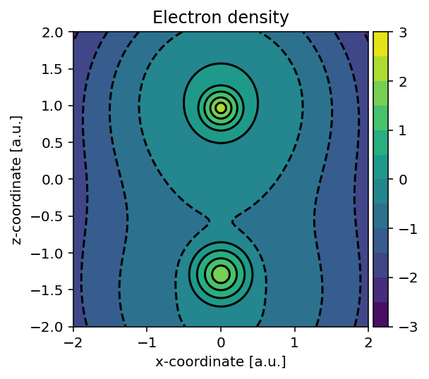
The pydft.DFT class exposes its internal matrices and a number of useful functions which we can readily use to interpret its operation. Let us start by generating a plot of the electron density using the method pydft.DFT.get_density_at_points().

import numpy as np
from pydft import MoleculeBuilder, DFT
import matplotlib.pyplot as plt
from mpl_toolkits.axes_grid1 import make_axes_locatable

# perform DFT calculation on the CO molecule
co = MoleculeBuilder().from_name("CO")
dft = DFT(co, basis='sto3g')
en = dft.scf(1e-6, verbose=False)

# generate grid of points and calculate the electron density for these points
sz = 4      # size of the domain
npts = 100  # number of sampling points per cartesian direction

# produce meshgrid for the xz-plane
x = np.linspace(-sz/2,sz/2,npts)
zz, xx = np.meshgrid(x, x, indexing='ij')
gridpoints = np.zeros((zz.shape[0], xx.shape[1], 3))
gridpoints[:,:,0] = xx
gridpoints[:,:,2] = zz
gridpoints[:,:,1] = np.zeros_like(xx) # set y-values to 0
gridpoints = gridpoints.reshape((-1,3))

# calculate (logarithmic) scalar field and convert if back to an 2D array
density = dft.get_density_at_points(gridpoints)
density = np.log10(density.reshape((npts, npts)))

# build contour plot
fig, ax = plt.subplots(1,1, dpi=144, figsize=(4,4))
im = ax.contourf(x, x, density, levels=np.linspace(-3,3,13, endpoint=True))
ax.contour(x, x, density, colors='black', levels=np.linspace(-3,3,13, endpoint=True))
ax.set_aspect('equal', 'box')
ax.set_xlabel('x-coordinate [a.u.]')
ax.set_ylabel('z-coordinate [a.u.]')
divider = make_axes_locatable(ax)
cax = divider.append_axes('right', size='5%', pad=0.05)
fig.colorbar(im, cax=cax, orientation='vertical')
ax.set_title('Electron density')

Running the above script yields the electron density.

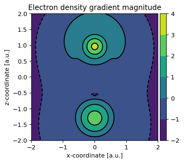
Using largely the same code, we can also readily build the electron density gradient magnitude using pydft.DFT.get_gradient_at_points().

import numpy as np
from pydft import MoleculeBuilder, DFT
import matplotlib.pyplot as plt
from mpl_toolkits.axes_grid1 import make_axes_locatable

# perform DFT calculation on the CO molecule
co = MoleculeBuilder().from_name("CO")
dft = DFT(co, basis='sto3g')
en = dft.scf(1e-6, verbose=False)

# generate grid of points and calculate the electron density for these points
sz = 4      # size of the domain
npts = 100  # number of sampling points per cartesian direction

# produce meshgrid for the xz-plane
x = np.linspace(-sz/2,sz/2,npts)
zz, xx = np.meshgrid(x, x, indexing='ij')
gridpoints = np.zeros((zz.shape[0], xx.shape[1], 3))
gridpoints[:,:,0] = xx
gridpoints[:,:,2] = zz
gridpoints[:,:,1] = np.zeros_like(xx) # set y-values to 0
gridpoints = gridpoints.reshape((-1,3))

# calculate (logarithmic) scalar field and convert if back to an 2D array
gradient = np.linalg.norm(dft.get_gradient_at_points(gridpoints), axis=1)
gradient = np.log10(gradient.reshape((npts, npts)))

# build contour plot
fig, ax = plt.subplots(1,1, dpi=144, figsize=(4,4))
im = ax.contourf(x, x, gradient, levels=np.linspace(-2,4,7, endpoint=True))
ax.contour(x, x, gradient, colors='black', levels=np.linspace(-2,4,7, endpoint=True))
ax.set_aspect('equal', 'box')
ax.set_xlabel('x-coordinate [a.u.]')
ax.set_ylabel('z-coordinate [a.u.]')
divider = make_axes_locatable(ax)
cax = divider.append_axes('right', size='5%', pad=0.05)
fig.colorbar(im, cax=cax, orientation='vertical')
ax.set_title('Electron density gradient magnitude')

Adjusting grid and discretization schemes

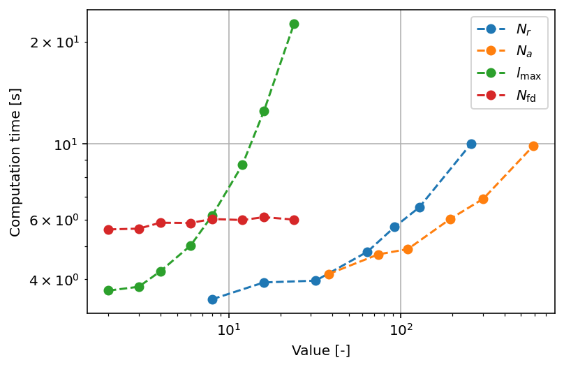
By default, PyDFT uses 32 radial grid points and 110 angular grid points per atom. To calculate the Hartree potential, the electron density is projected onto spherical harmonics with a maximum angular momentum of \(l_{\text{max}} = 8\). The finite-difference discretization scheme used to solve the Poisson equation uses 7 adjacent points. All these settings can be adjusted to potentially reduce computational time or to increase upon the accuracy. In the following subsections, this is explored in more detail. In the graph below, a visual summary of the scaling of the parameters in terms of computing time is provided.

Number of radial shells

In the listing below, the scaling with respect to the number of radial shells is shown. It can be readily seen that there are no more significant changes in the total electronic energy after \(N_{r} = 64\). On the basis of these results, it can be found that the computation time scales with \(t \propto N_{r}^{0.3725}\).

\(N_{r}\)	Energy [Ht]	Computation Time (s)
8	-114.0908	3.4304
16	-111.0566	3.6955
32	-111.1468	4.1970
64	-111.1495	4.9463
92	-111.1495	5.5899
128	-111.1495	6.5389
256	-111.1495	10.0511

Number of angular grid points

PyDFT uses by default 110 angular points per spherical shell. From the listing below, it can be seen that this yields decent accuracy in terms of energy, though the accuracy can be improved a bit further by using 194 or more angular points. On the basis of these results, it can be found that the computation time scales with \(t\propto N_{r}^{0.3344}\).

\(N_{a}\)	Energy	Computation Time (s)
38	-111.1226	4.1232
74	-111.1698	4.8680
110	-111.1495	5.4705
194	-111.1503	6.3094
302	-111.1503	7.0128
590	-111.1503	10.1610

Maximum angular momentum

For the calculation of the Hartree potential, the electron density is projected per radial shell onto spherical harmonics. The highest angular momentum used for the projection is determined by the lmax parameter, which by default is set to \(l_{\text{max}} =8\). Increasing this value further shows some irregularities in terms of the energy, which are assigned to increased numerical noise in the linear expansion coefficients used in the expansion scheme. The total number of spherical harmonics used scales with \(N_{\text{sh}} \propto l_{\text{max}}^{2}\), hence we see somewhat steeper scaling in terms of computational time for this parameter. On the basis of these results, it can be found that the computation time scales with \(t\propto l_{\text{max}}^{1.064}\).

It is relevant to mention that the original paper of Becke mentions that the ideal value for \(l_{\text{max}} \approx l_{\text{quad}}/2\) which yields \(l_{\text{max}}\) values of 5, 8, 11 and 14 for 50, 110, 194 and 302 angular points.

\(l_{\text{max}}\)	Energy	Computation Time (s)
2	-111.0728	3.7725
3	-111.1175	4.0743
4	-111.1412	4.4981
6	-111.1511	4.9934
8	-111.1503	6.0379
12	-111.1489	8.5445
16	-111.1489	12.2454
24	-111.0209	22.8109

Number discretization points

When calculating the Hartree potential, a second-order differential equation is solved for all spherical shells and for each spherical harmonic. This second-order differential equation is solved using a finite-difference approximation. For this finite-difference approximation, the number of points used to establish the first- and second-order derivatives can be set. In the following analysis, we examine the total electronic energy and computation time as functions of the number of discretization points. It is evident that beyond 7 discretization points, the total electronic energy remains unchanged. This is because the coefficients associated with points farther from the point of interest—where the derivative is calculated—become increasingly smaller. Consequently, the contribution of distant points diminishes rapidly, rendering expansions to a higher number of discretization points inefficient. Additionally, we observe minimal variation in computation time, which can be attributed to the exceptional efficiency of solving linear matrix equations. As a result, this aspect is not a significant computational bottleneck in the code.

\(N_{\text{fd}}\)	Energy	Computation Time (s)
3	-111.1028	5.8947
5	-111.1501	5.7674
7	-111.1503	6.3035
9	-111.1503	5.9776
11	-111.1503	5.8185
13	-111.1503	5.7800
15	-111.1503	5.8533
17	-111.1503	5.8799

Reproducing analysis

To reproduce the analysis, one can use the script as found below.

import numpy as np
from pydft import MoleculeBuilder, DFT
import matplotlib.pyplot as plt
import time

def main():
    # perform DFT calculation on the CO molecule
    co = MoleculeBuilder().from_name("CO")
    
    plt.figure(dpi=144)
    
    # explore scaling with number of radial shells
    t = []
    print('Spherical shells')
    nvals = [8,16,32,64,92,128,256]
    for n in nvals:
        st = time.time()
        dft = DFT(co, basis='sto3g', nshells=n)
        en = dft.scf(1e-6, verbose=False)
        dt = time.time() - st
        t.append(dt)
        print("%3i %12.4f %5.4f" % (n, en, dt))
    print()
    
    plt.loglog(nvals, t, 'o--', label=r'$N_{r}$')
    
    # explore scaling with number of angular points
    t = []    
    print('Angular points')
    avals = [38,74,110,194,302,590]
    for a in avals:
        st = time.time()
        dft = DFT(co, basis='sto3g', nshells=64, nangpts=a)
        en = dft.scf(1e-6, verbose=False)
        dt = time.time() - st
        t.append(dt)
        print("%3i %12.4f %5.4f" % (a, en, dt))
    print()
        
    plt.loglog(avals, t, 'o--', label=r'$N_{a}$')
        
    # explore scaling with lmax value
    t = []
    print('Lmax value')
    lvals = [2,3,4,6,8,12,16,24]
    for lmax in lvals:
        st = time.time()
        dft = DFT(co, basis='sto3g', nshells=64, nangpts=590, lmax=lmax)
        en = dft.scf(1e-6, verbose=False)
        dt = time.time() - st
        t.append(dt)
        print("%3i %12.4f %5.4f" % (lmax, en, dt))
    print()
    
    plt.loglog(lvals, t, 'o--', label=r'$l_{\text{max}}$')
    
    # explore scaling with number of discretization points used in the
    # finite difference scheme to construct the Hartree potential
    t = []
    print('Number of finite difference coefficients')
    fdvals = [3,5,7,9,11,13,15,17]
    for fd in fdvals:
        st = time.time()
        dft = DFT(co, basis='sto3g', nshells=64, nangpts=194, fdpts=fd)
        en = dft.scf(1e-6, verbose=False)
        dt = time.time() - st
        t.append(dt)
        print("%3i %12.4f %5.4f" % (fd, en, dt))
    print()
        
    plt.loglog(lvals, t, 'o--', label=r'$N_{\text{fd}}$')
    plt.grid()
    plt.xlabel('Value [-]')
    plt.ylabel('Computation time [s]')
    plt.legend()

if __name__ == '__main__':
    main()

Self-consistent field matrices

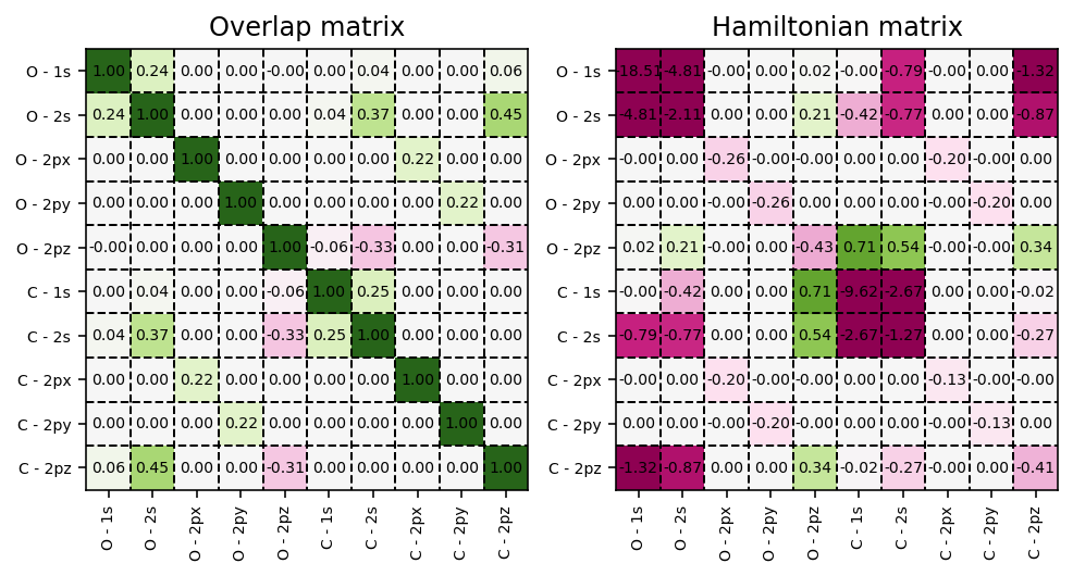
To obtain any of the matrices used in the self-consistent field procedure, we can invoke the pydft.DFT.get_data() method. For example, to visualize the overlap matrix \(\mathbf{S}\) and the Fock matrix \(\mathbf{F}\), we can use the script as found below.

import numpy as np
from pydft import MoleculeBuilder, DFT
import matplotlib.pyplot as plt

def main():
    # perform DFT calculation on the CO molecule
    co = MoleculeBuilder().from_name("CO")
    dft = DFT(co, basis='sto3g')
    en = dft.scf(1e-6, verbose=False)
    
    # build list of basis functions
    labels = []
    for a in co.get_atoms():
        for o in ['1s', '2s', '2px', '2py', '2pz']:
            labels.append('%s - %s' % (a[0],o))
    
    fig, ax = plt.subplots(1, 2, dpi=144, figsize=(8,4))
    plot_matrix(ax[0], dft.get_data()['S'], xlabels=labels, ylabels=labels, title='Overlap matrix')
    plot_matrix(ax[1], dft.get_data()['F'], xlabels=labels, ylabels=labels, title='Hamiltonian matrix')

def plot_matrix(ax, mat, xlabels=None, ylabels=None, title = None, xlabelrot=90):
    """
    Produce plot of matrix
    """
    ax.imshow(mat, vmin=-1, vmax=1, cmap='PiYG')
    for i in range(mat.shape[0]):
        for j in range(mat.shape[1]):
            ax.text(i, j, '%.2f' % mat[j,i], ha='center', va='center',
                    fontsize=7)
    ax.set_xticks([])
    ax.set_yticks([])
    ax.hlines(np.arange(1, mat.shape[0])-0.5, -0.5, mat.shape[0] - 0.5,
              color='black', linestyle='--', linewidth=1)
    ax.vlines(np.arange(1, mat.shape[0])-0.5, -0.5, mat.shape[0] - 0.5,
              color='black', linestyle='--', linewidth=1)
    
    ax.set_xticks(np.arange(0, mat.shape[0]))
    if xlabels is not None:
        ax.set_xticklabels(xlabels, rotation=xlabelrot)
    ax.set_yticks(np.arange(0, mat.shape[0]))
    
    if ylabels is not None:
        ax.set_yticklabels(ylabels, rotation=0)
    ax.tick_params(axis='both', which='major', labelsize=7)
    
    if title is not None:
        ax.set_title(title)

if __name__ == '__main__':
    main()

Energy decomposition

The molecular matrices can be used to perform a so-called energy decomposition, i.e., decompose the total electronic energy into the kinetic, nuclear attraction, electron-electron repulsion and exchange-correlation energy.

import numpy as np
from pydft import MoleculeBuilder, DFT

co = MoleculeBuilder().from_name("CO")
dft = DFT(co, basis='sto3g')
en = dft.scf(1e-4, verbose=False)
print("Total electronic energy:     %12.6f Ht" % en)
print()

# retrieve molecular matrices
res = dft.get_data()
P = res['P']
T = res['T']
V = res['V']
J = res['J']

# calculate energy terms
Et = np.einsum('ji,ij', P, T)
Ev = np.einsum('ji,ij', P, V)
Ej = 0.5 * np.einsum('ji,ij', P, J)
Ex = res['Ex']
Ec = res['Ec']
Exc = res['Exc']
Enuc = res['enucrep']

print('Kinetic energy:              %12.6f Ht' % Et)
print('Nuclear attraction:          %12.6f Ht' % Ev)
print('Electron-electron repulsion: %12.6f Ht' % Ej)
print('Exchange energy:             %12.6f Ht' % (Ex))
print('Correlation energy:          %12.6f Ht' % (Ec))
print('Exchange-correlation energy: %12.6f Ht' % (Exc))
print('Nucleus-nucleus repulsion:   %12.6f Ht' % (Enuc))
print()
print('Sum: %12.6f Ht' % (Et + Ev + Ej + Exc + Enuc))

The above script yields the following output:

Total electronic energy:      -111.147096 Ht

Kinetic energy:                110.216045 Ht
Nuclear attraction:           -304.930390 Ht
Electron-electron repulsion:    75.597401 Ht
Exchange energy:               -12.055579 Ht
Correlation energy:             -1.232665 Ht
Exchange-correlation energy:   -13.288244 Ht
Nucleus-nucleus repulsion:      21.258092 Ht

Sum:  -111.147096 Ht

Kohn-Sham orbitals and their visualization

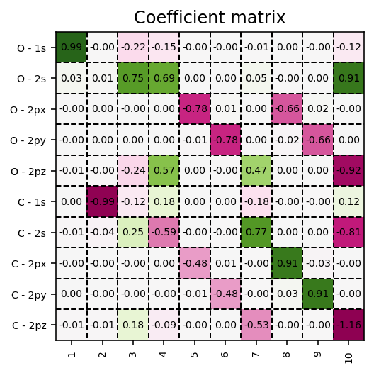
Within the Kohn-Sham approximation, the set of molecular orbitals that minimizes the total electronic energy are found via the diagonalization of the Fock matrix.

Coefficient matrix

These Kohn-Sham orbitals are encoded in the coefficient matrix which is extracted via the script below.

import numpy as np
from pydft import MoleculeBuilder, DFT
import matplotlib.pyplot as plt

def main():
    # perform DFT calculation on the CO molecule
    co = MoleculeBuilder().from_name("CO")
    dft = DFT(co, basis='sto3g')
    en = dft.scf(1e-6, verbose=False)
    
    # build list of basis functions
    labels = []
    for a in co.get_atoms():
        for o in ['1s', '2s', '2px', '2py', '2pz']:
            labels.append('%s - %s' % (a[0],o))
    
    fig, ax = plt.subplots(1, 1, dpi=144, figsize=(4,4))
    plot_matrix(ax, dft.get_data()['C'], xlabels=[str(i) for i in np.arange(1,11)], 
                ylabels=labels, title='Coefficient matrix')

def plot_matrix(ax, mat, xlabels=None, ylabels=None, title = None, xlabelrot=90):
    """
    Produce plot of matrix
    """
    ax.imshow(mat, vmin=-1, vmax=1, cmap='PiYG')
    for i in range(mat.shape[0]):
        for j in range(mat.shape[1]):
            ax.text(i, j, '%.2f' % mat[j,i], ha='center', va='center',
                    fontsize=7)
    ax.set_xticks([])
    ax.set_yticks([])
    ax.hlines(np.arange(1, mat.shape[0])-0.5, -0.5, mat.shape[0] - 0.5,
              color='black', linestyle='--', linewidth=1)
    ax.vlines(np.arange(1, mat.shape[0])-0.5, -0.5, mat.shape[0] - 0.5,
              color='black', linestyle='--', linewidth=1)
    
    ax.set_xticks(np.arange(0, mat.shape[0]))
    if xlabels is not None:
        ax.set_xticklabels(xlabels, rotation=xlabelrot)
    ax.set_yticks(np.arange(0, mat.shape[0]))
    
    if ylabels is not None:
        ax.set_yticklabels(ylabels, rotation=0)
    ax.tick_params(axis='both', which='major', labelsize=7)
    
    if title is not None:
        ax.set_title(title)

if __name__ == '__main__':
    main()

Contour plots

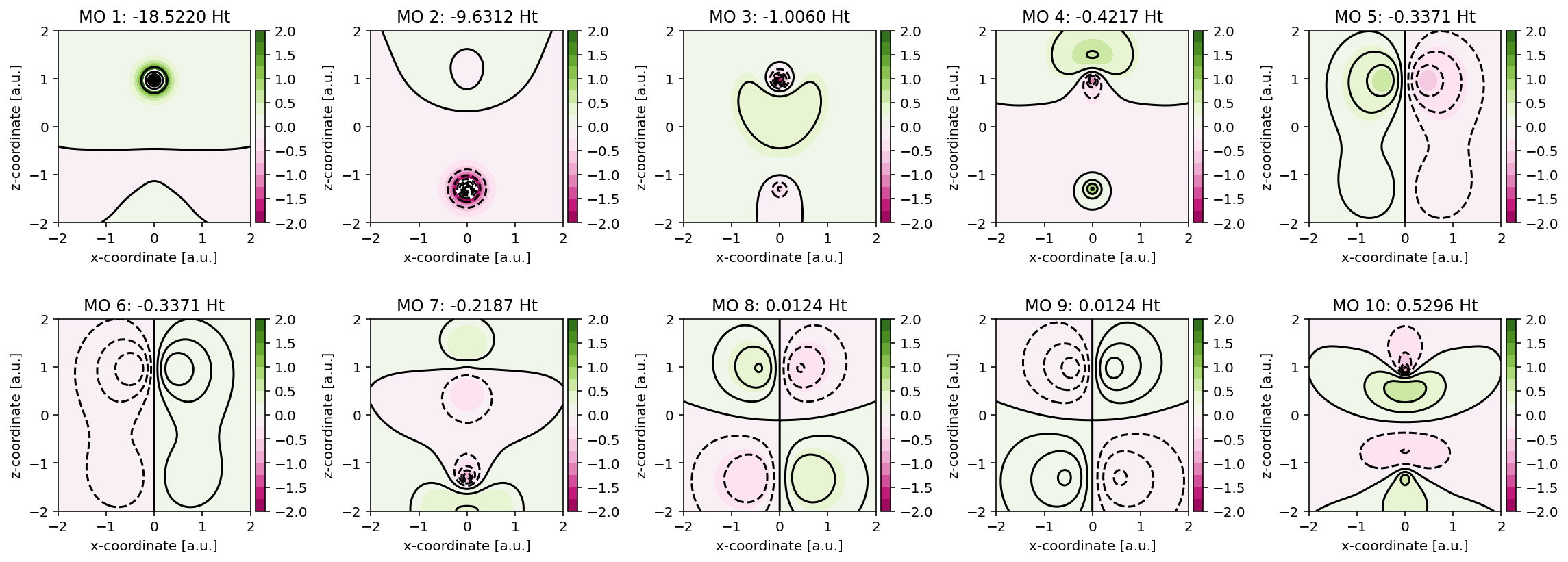
These orbitals can be readily visualized, as exemplified in the code below. Here, we make use of the pydft.MolecularGrid.get_amplitude_at_points() method. To use this method, we first have to retrieve the pydft.MolecularGrid object from the pydft.DFT class via its pydft.get_molgrid_copy() method.

import numpy as np
from pydft import MoleculeBuilder, DFT
import matplotlib.pyplot as plt
from mpl_toolkits.axes_grid1 import make_axes_locatable

def main():
    # perform DFT calculation on the CO molecule
    co = MoleculeBuilder().from_name("CO")
    dft = DFT(co, basis='sto3g')
    en = dft.scf(1e-6, verbose=False)
    
    # grab molecular orbital energies and coefficients
    orbc = dft.get_data()['C']
    orbe = dft.get_data()['orbe']  
    
    # generate grid of points and calculate the electron density for these points
    sz = 4      # size of the domain
    npts = 100  # number of sampling points per cartesian direction
    
    # produce meshgrid for the xz-plane
    x = np.linspace(-sz/2,sz/2,npts)
    zz, xx = np.meshgrid(x, x, indexing='ij')
    gridpoints = np.zeros((zz.shape[0], xx.shape[1], 3))
    gridpoints[:,:,0] = xx
    gridpoints[:,:,2] = zz
    gridpoints[:,:,1] = np.zeros_like(xx) # set y-values to 0
    gridpoints = gridpoints.reshape((-1,3))
    
    # grab a copy of the MolecularGrid object
    molgrid = dft.get_molgrid_copy()
    
    fig, ax = plt.subplots(2, 5, dpi=144, figsize=(16,6))
    for i in range(len(orbe)):
        m_ax = ax[i//5, i%5]
        
        # calculate field
        field = molgrid.get_amplitude_at_points(gridpoints, orbc[:,i]).reshape((npts, npts))
        
        # plot field
        levels = np.linspace(-2,2,17, endpoint=True)
        im = m_ax.contourf(x, x, field, levels=levels, cmap='PiYG')
        m_ax.contour(x, x, field, colors='black')
        m_ax.set_aspect('equal', 'box')
        m_ax.set_xlabel('x-coordinate [a.u.]')
        m_ax.set_ylabel('z-coordinate [a.u.]')
        divider = make_axes_locatable(m_ax)
        cax = divider.append_axes('right', size='5%', pad=0.05)
        fig.colorbar(im, cax=cax, orientation='vertical')
        m_ax.set_title('MO %i: %6.4f Ht' % (i+1, orbe[i]))

    plt.tight_layout()

if __name__ == '__main__':
    main()

See also

To get a better impression of the three-dimensional shape of the molecular orbitals, it is recommended to produce isosurfaces rather than contour plots.

Isosurfaces

Generating an isosurface is very similar to generating a contour plot, but with the notable difference that the orbital has to be sampled in three-dimensional space. In the script below, an example is provided for one of the \(1\pi\) orbitals of CO. Observe that for generating an isosurface, the algorithm has to be executed twice, once for the positive lobe and once for the negative lobe. The isosurfaces are stored in so-called Polygon File Format files which can be used in your favorite rendering program.

Note

Isosurface generation requires the PyTessel package to be installed. More information can be found here.

import numpy as np
from pydft import MoleculeBuilder, DFT
from pytessel import PyTessel

def main():
    # perform DFT calculation on the CO molecule
    co = MoleculeBuilder().from_name("CO")
    dft = DFT(co, basis='sto3g')
    en = dft.scf(1e-4, verbose=False)
        
    # grab a copy of the MolecularGrid object and of the coefficient matrix
    molgrid = dft.get_molgrid_copy()
    orbc = dft.get_data()['C']

    sz = 10     # size of the domain
    npts = 50   # number of sampling points per cartesian direction

    build_isosurface('1pi_pos.ply', molgrid, orbc[:,4], 0.03, sz, npts)
    build_isosurface('1pi_neg.ply', molgrid, orbc[:,4], -0.03, sz, npts)

def build_isosurface(filename, molgrid, coeff, isovalue, sz, npts):
    # produce meshgrid for the unit cell
    x = np.linspace(-sz/2, sz/2, npts)
    zz, yy, xx = np.meshgrid(x, x, x, indexing='ij')
    N = len(x)
    gridpoints = np.zeros((N, N, N, 3))
    gridpoints[:,:,:,0] = xx
    gridpoints[:,:,:,1] = yy
    gridpoints[:,:,:,2] = zz
    gridpoints = gridpoints.reshape((-1,3))

    # build isosurface
    scalarfield = molgrid.get_amplitude_at_points(gridpoints, coeff).reshape(npts, npts, npts)
    unitcell = np.diag(np.ones(3) * sz)

    pytessel = PyTessel()
    vertices, normals, indices = pytessel.marching_cubes(scalarfield.flatten(), scalarfield.shape, unitcell.flatten(), isovalue)
    pytessel.write_ply(filename, vertices, normals, indices)

if __name__ == '__main__':
    main()

Analyzing the Becke grid

All numerical integrations are performed by means of Gauss-Chebychev and Lebedev quadrature using the Becke grid.

Atomic fuzzy cells

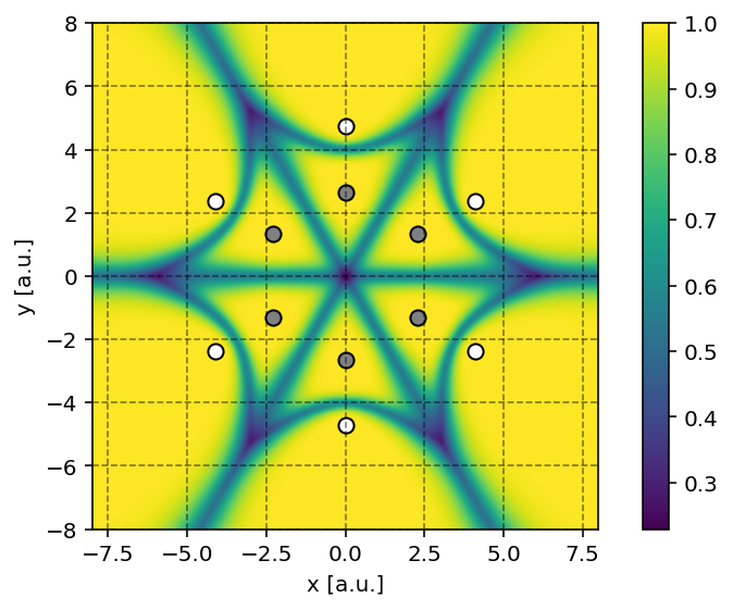
It is possible to produce a contour plot of the fuzzy cells (molecular weights) on a plane using the pydft.MolecularGrid.calculate_weights_at_points() method. An example is provided below.

from pydft import MolecularGrid
from pyqint import MoleculeBuilder
import numpy as np
import matplotlib.pyplot as plt

# construct molecule
mol = MoleculeBuilder().from_name('benzene')
cgfs, atoms = mol.build_basis('sto3g')

# construct molecular grid
molgrid = MolecularGrid(atoms, cgfs)

# produce grid of sampling points to calculate the atomic
# weight coefficients for
N = 150
sz = 8
x = np.linspace(-sz,sz,N)
xv,yv = np.meshgrid(x,x)
points = np.array([[x,y,0] for x,y in zip(xv.flatten(),yv.flatten())])

# calculate the atomic weights
mweights = molgrid.calculate_weights_at_points(points, k=3)

# plot the atomic weights
plt.figure(dpi=144)
plt.imshow(np.max(mweights,axis=0).reshape((N,N)),
           extent=(-sz,sz,-sz,sz), interpolation='bicubic')
plt.xlabel('x [a.u.]')
plt.ylabel('y [a.u.]')
plt.colorbar()
plt.grid(linestyle='--', color='black', alpha=0.5)

# add the atoms to the plot
r = np.zeros((len(atoms), 3))
for i,at in enumerate(atoms):
    r[i] = at[0]
plt.scatter(r[0:6,0], r[0:6,1], s=50.0, color='grey', edgecolor='black')
plt.scatter(r[6:12,0], r[6:12,1], s=50.0, color='white', edgecolor='black')

plt.tight_layout()

In the script above, we color every point by the maximum value for each of the atomic weights. When this maximum value is one, this implies that the grid point belongs to a single atom. When multiple atoms ‘share’ a grid point, the maximum value among the atomic weights will be lower than one.

Note

Producing such a contour plot is only meaningful for planar molecules such as benzene. For more complex molecules such as methane, it is rather difficult to make sense of the fuzzy cells upon projection on a plane.

Grid points

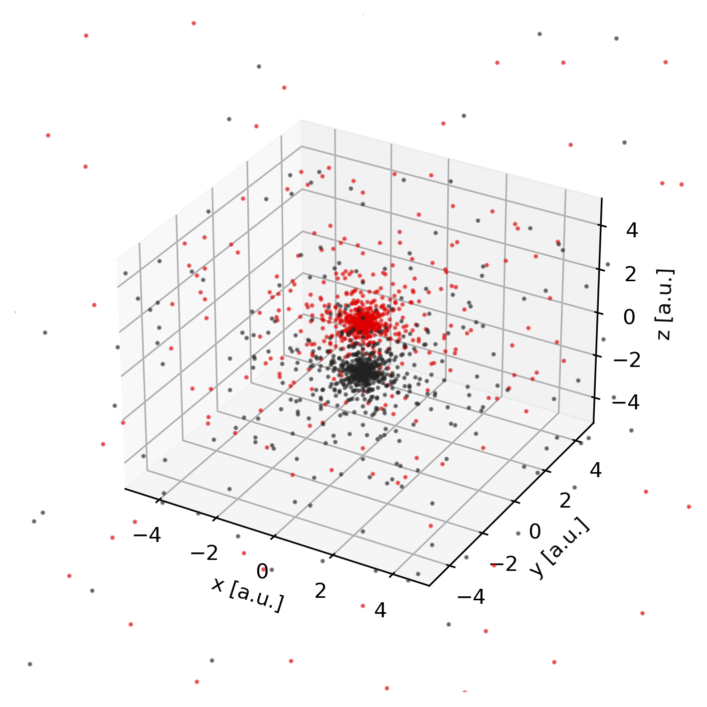
To obtain the set of grid points on which the numerical integration (quadrature), is performed, we can invoke the pydft.MolecularGrid.get_grid_coordinates() method.

from pydft import MolecularGrid
from pyqint import MoleculeBuilder
import matplotlib.pyplot as plt

# construct molecule
mol = MoleculeBuilder().from_name('co')
cgfs, atoms = mol.build_basis('sto3g')

# construct molecular grid
molgrid = MolecularGrid(atoms, cgfs, nshells=16, nangpts=74)
molgrid.initialize()

# obtain the grid points
gridpoints = molgrid.get_grid_coordinates()

# plot the atomic weights
colors = '#DD0000', '#222222'
fig = plt.figure(dpi=300, figsize=(8,6))
ax = fig.add_subplot(projection='3d')
for i in range(0, len(gridpoints)):
    ax.scatter(gridpoints[i][:,0], gridpoints[i][:,1], gridpoints[i][:,2],
               s = 1.5, alpha=0.5, color=colors[i])

# set axes
ax.set_xlim(-5,5)
ax.set_ylim(-5,5)
ax.set_zlim(-5,5)
ax.set_xlabel('x [a.u.]')
ax.set_ylabel('y [a.u.]')
ax.set_zlabel('z [a.u.]')
ax.set_box_aspect(aspect=None, zoom=0.8)

Hartree potential

The Hartree potential is calculated from the electron density distribution using the Poisson equation.

Projection onto spherical harmonics

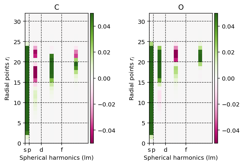
The Poisson equation is solved on the atomic grid by first projecting the electron density onto the spherical harmonics such that the following equation holds.

\[\rho(r_{k}, \Omega) = \sum_{lm} \rho_{klm} Y_{lm}\]

where \(\rho(r_{k}, \Omega)\) is the electron density at radius \(r_{k}\), \(\rho_{klm}\) the linear expansion coefficient at position \(r_{k}\) for the spherical harmonic \(lm\) and \(Y_{lm}\) a spherical harmonic with quantum numbers \(l\) and \(m\).

We can readily visualize and interpret this projection using the pydft.MolecularGrid.get_rho_lm_atoms() as shown by the script below.

import numpy as np
from pydft import MoleculeBuilder, DFT
import matplotlib.pyplot as plt
from mpl_toolkits.axes_grid1 import make_axes_locatable

def main():
    # perform DFT calculation on the CO molecule
    co = MoleculeBuilder().from_name("CO")
    dft = DFT(co, basis='sto3g')
    en = dft.scf(1e-6, verbose=False)
    
    # get the projection onto the spherical harmonics
    lmprojection = dft.get_molgrid_copy().get_rho_lm_atoms()
    
    fig, ax = plt.subplots(1, 2, dpi=144, figsize=(6,4))
    plot_spherical_harmonic_projection(ax[1], fig, lmprojection[0], title='O')
    plot_spherical_harmonic_projection(ax[0], fig, lmprojection[1], title='C')
    plt.tight_layout()

def plot_spherical_harmonic_projection(ax, fig, mat, minval=5e-2, title=None):
    im = ax.imshow(np.flip(mat, axis=0), origin='lower', cmap='PiYG', vmin=-minval,vmax=minval)
    ax.grid(linestyle='--', color='black', alpha=0.8)
    ax.set_xticks([-0.5,0.5,3.5,8.5,15.5], labels=['s','p','d','f','g'])
    ax.set_yticks(np.arange(0, mat.shape[0], 5)-0.5, 
                  labels=np.arange(0, mat.shape[0], 5))
    ax.set_ylabel('Radial points $r_{i}$')
    ax.set_xlim(-.5,15)
    ax.set_xlabel('Spherical harmonics (lm)')
    divider = make_axes_locatable(ax)
    cax = divider.append_axes('right', size='5%', pad=0.05)
    fig.colorbar(im, cax=cax, orientation='vertical')
    
    if title is not None:
        ax.set_title(title)

if __name__ == '__main__':
    main()

Exchange-correlation functional

The exchange and correlation potentials depend on the electron density and once the latter has been established, we can readily visualize these potentials.

Visualizing exchange potential

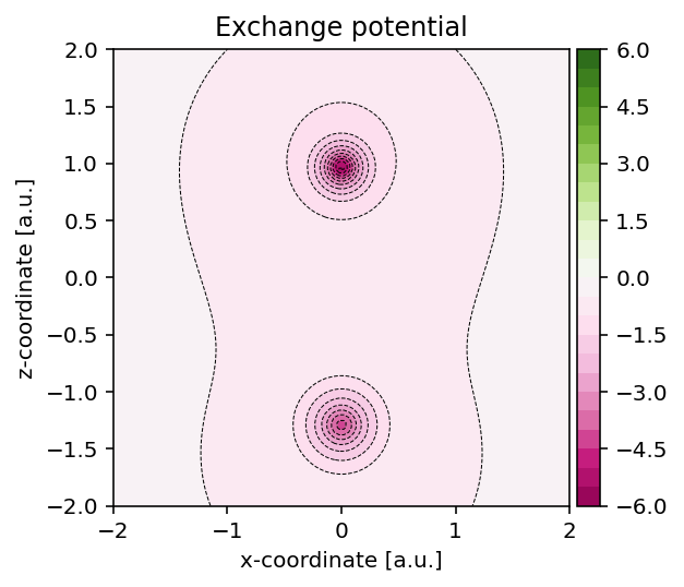
To construct the exchange potential at arbitrary grid points, we can use the script as shown below which uses the pydft.MolecularGrid.get_exchange_potential_at_points() method.

from pydft import DFT
from pyqint import MoleculeBuilder
import numpy as np
import matplotlib.pyplot as plt
from mpl_toolkits.axes_grid1 import make_axes_locatable

# perform DFT calculation on the CO molecule
co = MoleculeBuilder().from_name("CO")
dft = DFT(co, basis='sto3g')
en = dft.scf(1e-6, verbose=False)

# grab molecular orbital energies and coefficients
orbc = dft.get_data()['C']
orbe = dft.get_data()['orbe']  

# generate grid of points and calculate the electron density for these points
sz = 4      # size of the domain
npts = 100  # number of sampling points per cartesian direction

# produce meshgrid for the xz-plane
x = np.linspace(-sz/2,sz/2,npts)
zz, xx = np.meshgrid(x, x, indexing='ij')
gridpoints = np.zeros((zz.shape[0], xx.shape[1], 3))
gridpoints[:,:,0] = xx
gridpoints[:,:,2] = zz
gridpoints[:,:,1] = np.zeros_like(xx) # set y-values to 0
gridpoints = gridpoints.reshape((-1,3))

# grab a copy of the MolecularGrid object
molgrid = dft.get_molgrid_copy()

# construct exchange potential
field = molgrid.get_exchange_potential_at_points(gridpoints, dft.get_data()['P'])
field = field.reshape((npts, npts))

# plot field
fig, ax = plt.subplots(1, 1, dpi=144, figsize=(4,4))
levels = np.linspace(-6,6,25, endpoint=True)
im = ax.contourf(x, x, field, levels=levels, cmap='PiYG')
ax.contour(x, x, field, levels=levels, colors='black', linewidths=0.5)
ax.set_aspect('equal', 'box')
ax.set_xlabel('x-coordinate [a.u.]')
ax.set_ylabel('z-coordinate [a.u.]')
divider = make_axes_locatable(ax)
cax = divider.append_axes('right', size='5%', pad=0.05)
fig.colorbar(im, cax=cax, orientation='vertical')
ax.set_title('Exchange potential')

Visualizing correlation potential

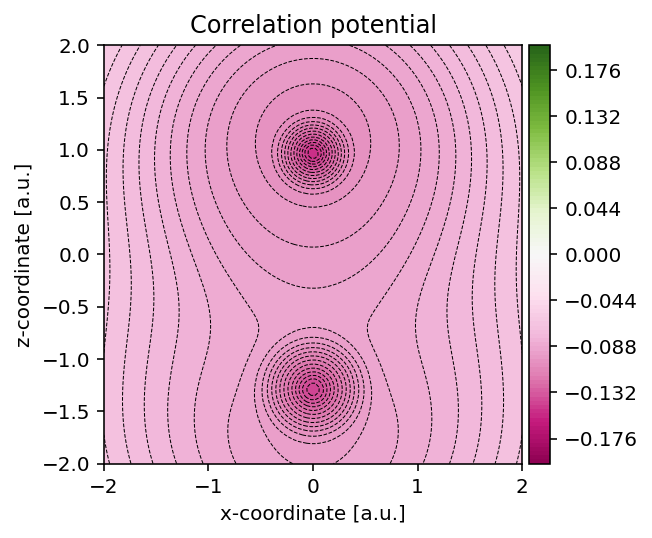
In a similar fashion as for the exchange potential, we can use the method pydft.MolecularGrid.get_correlation_potential_at_points() to obtain the correlation potential field.

from pydft import DFT
from pyqint import MoleculeBuilder
import numpy as np
import matplotlib.pyplot as plt
from mpl_toolkits.axes_grid1 import make_axes_locatable

# perform DFT calculation on the CO molecule
co = MoleculeBuilder().from_name("CO")
dft = DFT(co, basis='sto3g')
en = dft.scf(1e-6, verbose=False)

# grab molecular orbital energies and coefficients
orbc = dft.get_data()['C']
orbe = dft.get_data()['orbe']  

# generate grid of points and calculate the electron density for these points
sz = 4      # size of the domain
npts = 100  # number of sampling points per cartesian direction

# produce meshgrid for the xz-plane
x = np.linspace(-sz/2,sz/2,npts)
zz, xx = np.meshgrid(x, x, indexing='ij')
gridpoints = np.zeros((zz.shape[0], xx.shape[1], 3))
gridpoints[:,:,0] = xx
gridpoints[:,:,2] = zz
gridpoints[:,:,1] = np.zeros_like(xx) # set y-values to 0
gridpoints = gridpoints.reshape((-1,3))

# grab a copy of the MolecularGrid object
molgrid = dft.get_molgrid_copy()

# construct exchange potential
field = molgrid.get_correlation_potential_at_points(gridpoints, dft.get_data()['P'])
field = field.reshape((npts, npts))

# plot field
fig, ax = plt.subplots(1, 1, dpi=144, figsize=(4,4))
levels = np.linspace(-0.2,0.2,101, endpoint=True)
im = ax.contourf(x, x, field, levels=levels, cmap='PiYG')
ax.contour(x, x, field, levels=levels, colors='black', linewidths=0.5)
ax.set_aspect('equal', 'box')
ax.set_xlabel('x-coordinate [a.u.]')
ax.set_ylabel('z-coordinate [a.u.]')
divider = make_axes_locatable(ax)
cax = divider.append_axes('right', size='5%', pad=0.05)
fig.colorbar(im, cax=cax, orientation='vertical')
ax.set_title('Correlation potential')